Lesson 3
Computation graphs
Introduction
A computation graph shows a mathematical expression as a sequence of steps. The forward pass of logistic regression gives one small graph. The loss tensor(0.0852) shows how the values flow from the inputs to the output.
- Learning goal
Define a computation graph, read each node of a forward pass, and name the value that every symbol holds.
- Before you start
Lesson 2 on tensors. Basic Python variables and simple arithmetic.
Lesson plan
- Define a computation graph and name the role of each node and edge.
- Work through the forward pass of a logistic regression classifier.
- Compute the loss for a new set of values by hand, then check the answer.
What a computation graph is
A computation graph is a directed graph. It shows a mathematical expression as a sequence of steps. Each node holds a value. Each edge passes a value to the next operation.
In deep learning, the graph shows how the input becomes the output. The graph also gives the path for backpropagation. Backpropagation uses the graph to find the gradients of the loss.
A small network has a short graph. A large network has a long graph. The shape stays the same. Values flow from the inputs to the loss.
Worked example: a logistic regression forward pass
Logistic regression is a single-layer classifier. It gives a score between 0 and 1. Compare the score with the true label, 0 or 1, to compute the loss.
This program builds the graph for one example. Do not worry if not every part is clear. The point is the shape of the computation.
import torch.nn.functional as F

y  = torch.tensor([1.0])   # true label
x1 = torch.tensor([1.1])   # input feature
w1 = torch.tensor([2.2])   # weight parameter
b  = torch.tensor([0.0])   # bias unit

z = x1 * w1 + b          # net input
a = torch.sigmoid(z)     # activation and output

loss = F.binary_cross_entropy(a, y)
print(loss)

# Expected output:
# tensor(0.0852)
Read the graph node by node
The graph has one node for each value. The program runs the nodes from left to right. Follow the steps in order.
- Read
x1 = 1.1andw1 = 2.2from the input and parameter nodes. - Multiply them at the multiplication node:
1.1 * 2.2 = 2.42. - Add the bias
b = 0.0at the addition node:2.42 + 0.0 = 2.42. This sum is the net inputz. - Pass
zthrough the sigmoid node. The outputa = sigmoid(2.42) = 0.9183approximately. - Compare
awith the true labelyat the loss node. The loss istensor(0.0852).
What each symbol means
y- The true label. The value is
1.0for the positive class. The classifier must predict this value. x1- The input feature. The value is
1.1. A real model uses many features. w1- The weight for
x1. The value is2.2. Training changes this number. b- The bias unit. The value is
0.0. The bias moves the score up or down. z- The net input. The graph computes
z = x1 * w1 + b = 1.1 * 2.2 + 0.0 = 2.42. a- The activation and output. The sigmoid function maps
zto a value between 0 and 1. Herea = sigmoid(2.42) = 0.9183approximately. loss- The binary cross-entropy loss. It compares
awithy. The value istensor(0.0852).
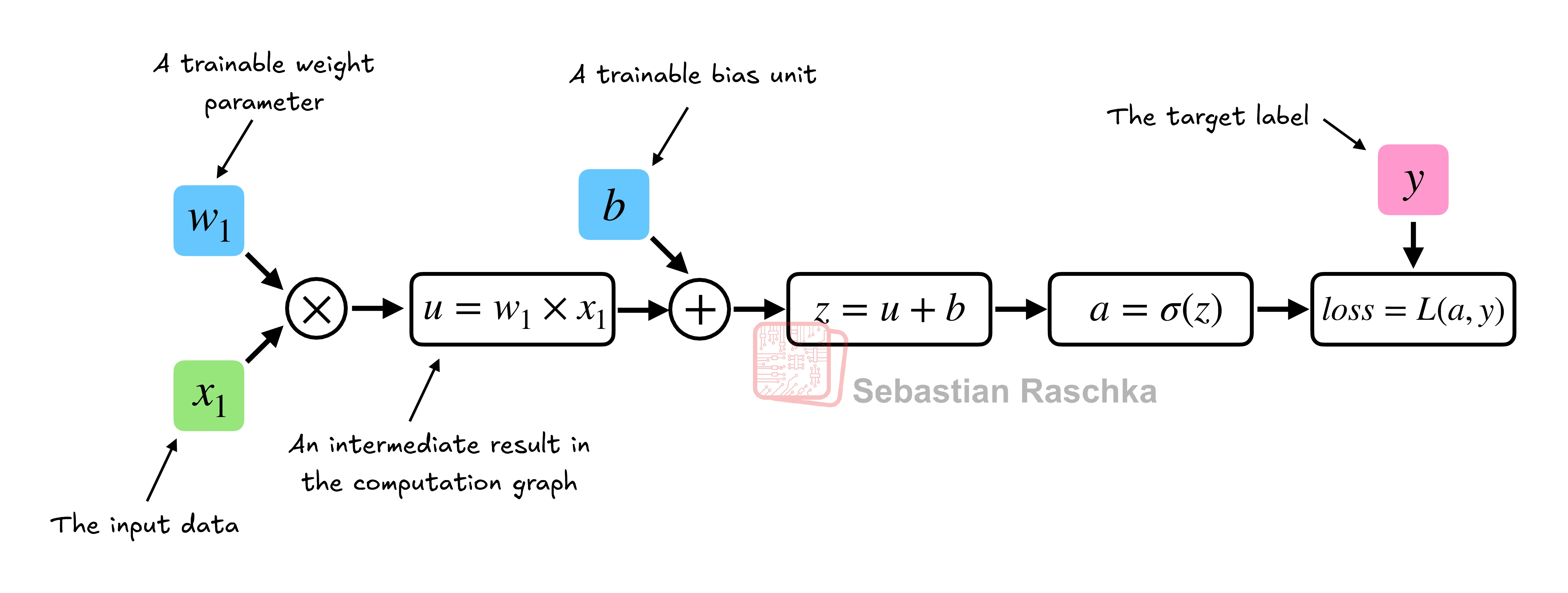
PyTorch builds this graph in the background. Later we use the graph to find the gradients of the loss with respect to the parameters. Then training can change the parameters. The next lesson explains this step.
Try it
Change x1 to 2.0 and w1 to 1.5. Keep b = 0.0 and y = 1.0. Compute z and the loss by hand. Then run the program and check your answer.
Reveal the worked answer
Step 1: compute the net input.
z = x1 * w1 + b = 2.0 * 1.5 + 0.0 = 3.0
Step 2: compute the activation.
a = sigmoid(3.0) = 0.9526 approximately.
Step 3: compute the loss. The true label is 1, so the loss is -ln(a).
loss = -ln(0.9526) = 0.0486 approximately.
import torch
import torch.nn.functional as F

y  = torch.tensor([1.0])
x1 = torch.tensor([2.0])
w1 = torch.tensor([1.5])
b  = torch.tensor([0.0])

z = x1 * w1 + b
a = torch.sigmoid(z)
loss = F.binary_cross_entropy(a, y)
print(loss)

# Expected output:
# tensor(0.0486)
The larger net input gives a smaller loss. The output a is closer to the true label, so the classifier is more confident.
Recap
A computation graph is a directed graph of a mathematical expression. Nodes hold values. Edges pass values between operations. The forward pass fills each node from left to right.
Logistic regression shows the idea in a small graph: inputs and weights multiply, the bias adds, sigmoid squashes, and the loss compares the output with the label. PyTorch builds the same graph in the background. In the next lesson, autograd uses the graph to compute gradients.
Reference: PyTorch in One Hour.