Lesson 4

Automatic differentiation

Why autograd needs requires_grad

Training changes parameters to lower a loss. A gradient measures how a small change in a parameter changes the loss. PyTorch can find gradients for you. However, it must first know which tensors to track.

A tensor with requires_grad=True asks PyTorch to track every operation that uses it. The result is a computation graph. The graph connects input values to the loss through the operations that created them.

Leaf tensors are the values that you create directly, such as weights and biases. PyTorch finds gradients for leaf tensors. A tensor without requires_grad does not need a gradient, so PyTorch can skip it.

The chain rule from right to left

Backpropagation uses the chain rule from calculus. The chain rule multiplies the local derivatives along a path. PyTorch applies the rule from right to left. It starts at the loss and moves back to the inputs.

This method is reverse-mode automatic differentiation. The forward pass builds the graph. The backward pass walks the graph in reverse and fills the gradient of each tracked leaf.

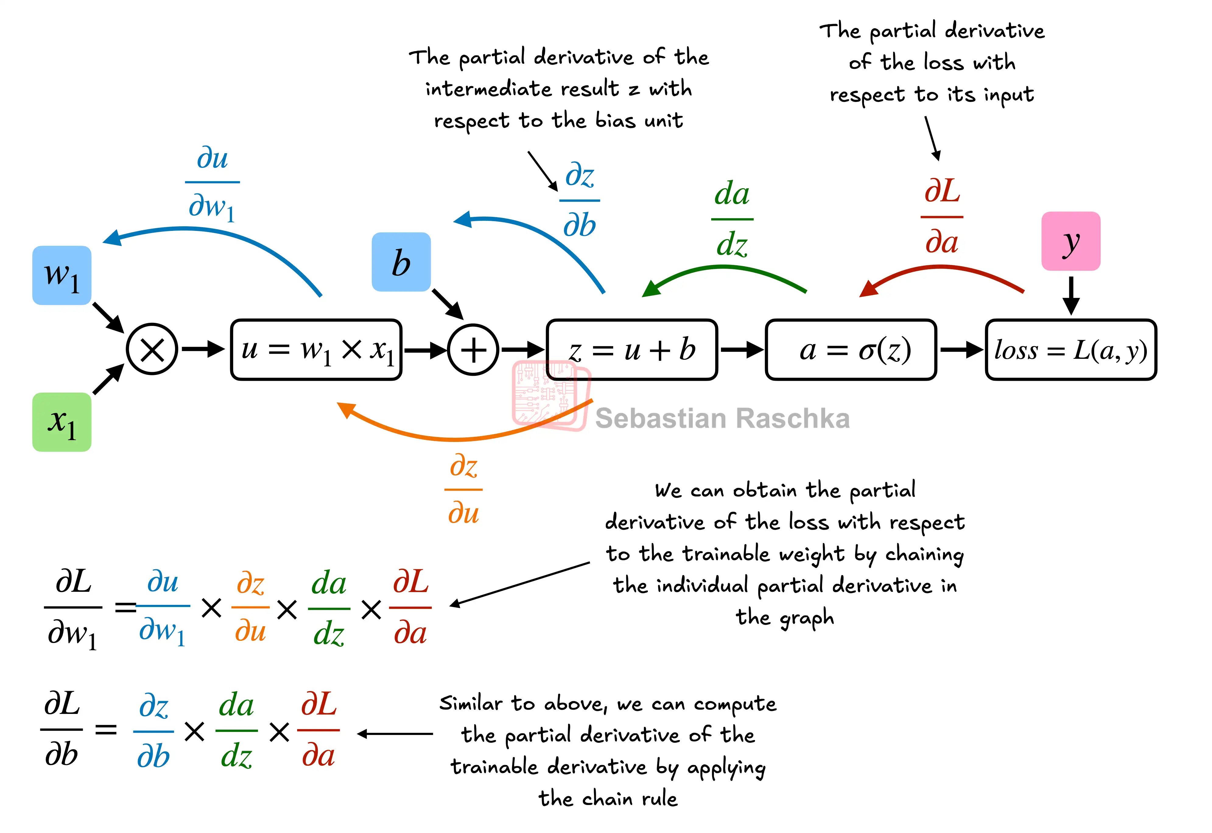
For a parameter w, the backward pass computes dL/dw as a product of local derivatives along the path from w to the loss. Each node supplies its own local derivative. PyTorch therefore does not need the full formula for the loss.

Reverse-mode automatic differentiation

Reverse mode makes one forward pass for the loss and then one backward pass for all parameters. This order is efficient when the loss is one scalar and the parameters are many. A model can have millions of parameters, so this order saves much work.

Partial derivatives and gradients

A partial derivative gives the rate of change of a function for one variable while the other variables stay fixed. Write the partial derivative of L with respect to w as dL/dw.

A gradient collects all partial derivatives of a function that has more than one input. The gradient is a vector. Each element tells how the loss responds to one parameter.

Gradient descent uses these values to lower the loss. It subtracts a small multiple of each gradient from the matching parameter. The gradient points uphill, so the subtraction moves the parameter downhill.

The grad() function

Autograd tracks every operation on tensors. It builds a computation graph in the background. Call the grad function to compute the gradient of the loss with respect to one parameter.

import torch.nn.functional as F
from torch.autograd import grad

y  = torch.tensor([1.0])
x1 = torch.tensor([1.1])
w1 = torch.tensor([2.2], requires_grad=True)
b  = torch.tensor([0.0], requires_grad=True)

z = x1 * w1 + b
a = torch.sigmoid(z)

loss = F.binary_cross_entropy(a, y)

grad_L_w1 = grad(loss, w1, retain_graph=True)
grad_L_b  = grad(loss, b,  retain_graph=True)

PyTorch destroys the graph after a gradient calculation by default. That action frees memory. Set retain_graph=True when you use the same graph again, as in this example.

print(grad_L_w1)
print(grad_L_b)

# Expected:
# (tensor([-0.0898]),)
# (tensor([-0.0817]),)

The grad function is useful for experiments and debugging. In a normal training loop, use the higher-level tools instead.

The .backward() method

Call .backward() on the loss. PyTorch then computes the gradients of all leaf nodes in the graph. Each leaf keeps its gradient in the .grad attribute.

loss.backward()

print(w1.grad)
print(b.grad)

# Expected:
# tensor([-0.0898])
# tensor([-0.0817])

PyTorch does the calculus for you through the .backward method. You usually do not compute derivatives or gradients by hand.

Gradients accumulate

PyTorch adds each new gradient to the value already in .grad. This behavior is useful when you combine several small batches. It is also a common bug. If you call backward() twice without a clear, .grad holds the sum of both gradients.

Training loops call optimizer.zero_grad() before the next backward pass. You can also set a gradient to None. Clear the old gradient unless you intend to accumulate it.

import torch

w = torch.tensor(2.0, requires_grad=True)

(w * 3).backward()            # w.grad is 3
(w * 3).backward()            # w.grad becomes 6
print(w.grad.item())          # Expected: 6.0

w.grad = None                 # clear the gradient
(w * 3).backward()
print(w.grad.item())          # Expected: 3.0

Try it

Let x = 3 and y = x² + 3x. Predict dy/dx by hand. Then compute it with grad() and with backward(), and confirm that both results match.

import torch
from torch.autograd import grad

x = torch.tensor(3.0, requires_grad=True)
y = x ** 2 + 3 * x

print(grad(y, x, retain_graph=True))  # Expected: (tensor(9.),)
y.backward()
print(x.grad.item())                  # Expected: 9.0

Recap

requires_grad=True marks a tensor for gradient tracking. PyTorch builds a computation graph during the forward pass. Reverse-mode autodiff applies the chain rule from right to left. The partial derivatives combine into one gradient vector. Use grad() for one value and backward() for all leaves. Clear accumulated gradients before each normal training step.

In the next lesson, neural networks collect many tracked parameters under one model. The gradient rule stays the same. Only the organization changes.

Reference: PyTorch autograd documentation.