Lesson 5
Multilayer neural networks
Introduction
A multilayer perceptron stacks linear layers with nonlinear activations. This lesson defines one with nn.Module, counts its trainable parameters, and reads its logits and probabilities.
- Learning goal
Define a network with nn.Module, count its trainable parameters, and read logits and probabilities from a forward pass.
- Before you start
Python classes, tensors, matrix multiplication, and the nn.Module container from Lesson 3.
Lesson plan
- Subclass nn.Module and define the layers in __init__ and the data flow in forward.
- Run the NeuralNetwork example, print its structure, and count 2213 trainable parameters.
- Inspect weights, run a forward pass, and convert logits to probabilities with softmax.
You only need Python classes, tensors, and the nn.Module container from Lesson 3. If class C(nn.Module): ... and forward are familiar, you are ready.
What a multilayer perceptron is
A neural network chains simple calculations. Each layer multiplies its input by a weight matrix and adds a bias vector. An activation function then adds nonlinearity. Stack two or more such layers, and the network can learn a complex mapping.
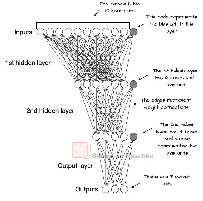
A multilayer perceptron is a fully connected network. Every node in one layer connects to every node in the next layer. A hidden layer is a layer between the input and the output. The network uses hidden layers to build intermediate features.
Figure 9 shows the example architecture. It has 50 input features, two hidden layers with 30 and 20 units, and 3 output scores.
Subclass nn.Module
PyTorch defines a network by subclassing torch.nn.Module. The base class holds layers and operations. It also keeps track of the model parameters.
Inside the subclass, define the layers in the __init__ constructor. Define the data flow in the forward method. That method shows how the input passes through the network. It forms the computation graph.
Do not write the backward method. PyTorch uses the computation graph to compute the gradients during training.
Define the layers and the forward pass
torch.nn.Sequential holds a series of layers. The layers run in order. The forward method then calls self.layers one time.
import torch

class NeuralNetwork(torch.nn.Module):
    def __init__(self, num_inputs, num_outputs):
        super().__init__()

        self.layers = torch.nn.Sequential(
            # 1st hidden layer
            torch.nn.Linear(num_inputs, 30),
            torch.nn.ReLU(),
            # 2nd hidden layer
            torch.nn.Linear(30, 20),
            torch.nn.ReLU(),
            # output layer
            torch.nn.Linear(20, num_outputs),
        )

    def forward(self, x):
        logits = self.layers(x)
        return logits
Sequential is optional
super().__init__() runs the setup code from nn.Module. It must run before you assign the submodules. Assign the layers to an attribute, such as self.layers. PyTorch then registers their weights and biases.
Sequential is a convenience. It makes a series of layers easy and it runs them in order. You can also store each layer in its own attribute and call them one by one in forward.
Print the model structure
Make a new network object with 50 inputs and 3 outputs. Print the object to see its layer order and shapes.
model = NeuralNetwork(50, 3)
print(model)
The output lists each child layer in order.
NeuralNetwork(
  (layers): Sequential(
    (0): Linear(in_features=50, out_features=30, bias=True)
    (1): ReLU()
    (2): Linear(in_features=30, out_features=20, bias=True)
    (3): ReLU()
    (4): Linear(in_features=20, out_features=3, bias=True)
  )
)
The indices 0 to 4 give the position of each layer inside Sequential. The first Linear maps 50 inputs to 30 hidden units. The final Linear maps 20 hidden units to 3 output scores.
Count the trainable parameters
A parameter with requires_grad=True is trainable. Training updates it. Sum the number of values in every trainable parameter.
num_params = sum(
    p.numel() for p in model.parameters() if p.requires_grad
)
print("Total number of trainable model parameters:", num_params)
Total number of trainable model parameters: 2213The trainable parameters live in the three nn.Linear layers. Each layer holds a weight matrix and a bias vector. The ReLU layers hold no parameters. Check the arithmetic:
- Layer 0: 30 times 50 weights plus 30 biases equals 1530.
- Layer 2: 20 times 30 weights plus 20 biases equals 620.
- Layer 4: 3 times 20 weights plus 3 biases equals 63.
The sum is 1530 + 620 + 63 = 2213. This value matches the printed count.
| Step | Code | Result |
|---|---|---|
| Instantiate | model = NeuralNetwork(50, 3) | Builds the layers with random weights. |
| Count | sum(p.numel() for p in model.parameters() if p.requires_grad) | 2213 trainable values. |
| Inspect | model.layers[0].weight.shape | torch.Size([30, 50]) |
The Linear layer
A linear layer multiplies the inputs by a weight matrix and adds a bias vector. Another name is a feedforward layer, or a fully connected layer. Read the first weight matrix. It is at index 0.
print(model.layers[0].weight)
print(model.layers[0].weight.shape)   # torch.Size([30, 50])
The weight matrix is 30 by 50. The rows are output units and the columns are input features. Read the bias with model.layers[0].bias. Its shape is torch.Size([30]).
Weights and biases in torch.nn.Linear have requires_grad=True by default. This setting makes them trainable.
Random initialization
PyTorch starts the weights with small random numbers. The numbers change each time you make the network. Random start values break symmetry during training. Without them, the nodes do the same operations and updates. The network then cannot learn complex mappings.
Make the random numbers repeatable with torch.manual_seed.
torch.manual_seed(123)
model = NeuralNetwork(50, 3)
print(model.layers[0].weight)
Run this code again, and you get the same numbers. The seed fixes the random generator. A fixed seed helps you compare runs. A different seed gives different start values.
The forward pass
Make one random input with 50 features. The network gives three scores.
torch.manual_seed(123)

X = torch.rand((1, 50))
out = model(X)
print(out)
tensor([[-0.1262, 0.1080, -0.1792]], grad_fn=<AddmmBackward0>)The call model(x) runs the forward pass. The input data passes through all layers: the input layer, the hidden layers, and the output layer. The three numbers are the scores of the three output nodes.
The output has grad_fn=<AddmmBackward0>. This value names the last function that made the tensor. Addmm means matrix multiply, mm, and addition, Add. PyTorch uses this information to compute the gradients during backpropagation.
Inference with no_grad
For inference, you do not need the graph. The graph costs memory and compute. Use the torch.no_grad() context manager.
with torch.no_grad():
    out = model(X)
print(out)
tensor([[-0.1262, 0.1080, -0.1792]])The numbers are the same. The output now has no grad_fn. Wrap evaluation and prediction code in torch.no_grad() to save memory.
Logits and softmax
The model returns the outputs of the last layer. These outputs are the logits. The model does not pass them to a nonlinear activation. The usual loss functions combine softmax, or sigmoid for binary tasks, with the negative log-likelihood loss in one class. This combination is fast and stable.
To get class probabilities, call softmax yourself.
with torch.no_grad():
    out = torch.softmax(model(X), dim=1)
print(out)
tensor([[0.3113, 0.3934, 0.2952]])The values are class probabilities. They sum to 1. The values are near equal for this random input. This result is expected for a model without training.
Common pitfalls
- Call
super().__init__()before you define the child layers. - Define the layers in
__init__, not insideforward. Otherwise new weights appear on every call. - Do not apply softmax before
nn.CrossEntropyLoss; that loss expects raw logits. - Keep one seed while you compare runs. A forgotten seed makes the weights differ each time.
- Use
torch.no_grad()for inference. A missing context costs memory and compute.
Try it
Change the network to accept 10 input features and produce 4 output scores. Use hidden layers with 8 and 6 units. What is the printed parameter count?
Reveal the worked answer
import torch

class NeuralNetwork(torch.nn.Module):
    def __init__(self, num_inputs, num_outputs):
        super().__init__()
        self.layers = torch.nn.Sequential(
            torch.nn.Linear(num_inputs, 8),
            torch.nn.ReLU(),
            torch.nn.Linear(8, 6),
            torch.nn.ReLU(),
            torch.nn.Linear(6, num_outputs),
        )

    def forward(self, x):
        return self.layers(x)

model = NeuralNetwork(10, 4)
num_params = sum(p.numel() for p in model.parameters() if p.requires_grad)
print(num_params)

# Expected: 170
The three linear layers hold 88, 54, and 28 trainable values. The total is 88 + 54 + 28 = 170.
Recap
Subclass nn.Module to define a network. Put the layers in __init__ and the data flow in forward. Sequential runs a series of layers in order. The linear layers hold the trainable weights and biases. In this example the count is 2213.
A forward pass returns logits with a grad_fn. Use torch.no_grad() for inference. Apply softmax yourself to turn logits into probabilities. In the next lesson, data loaders will feed batches to this network.
Reference: PyTorch nn documentation.